Lam Tran

Seeking internships for Summer 2027Summer ’27

BOSTON UNIVERSITYB.A. CS & ECONOMICS ’28GPA 3.50DEAN’S LIST ×2

Lam Tran

I build compilers, exchanges and pricing engines, then measure them.

I work from first principles in C++23 and Python, and check each system against something stronger: a slower oracle, a proof, a byte-exact replay.

Seeking Summer 2027 internships · software engineering and quant / trading systemsSeeking Summer 2027 SWE + quant internships

Loading the room

SIX SYSTEMS · STRONGEST NUMBER EACH

  1. FIG. 1 loom measured result 114.8 GFLOP/s · SGEMM, 1 threadSGEMM 114.8 GFLOP/s
  2. FIG. 2 sim-ex measured result 2.99M cmd/s · one M3 Pro core2.99M cmd/s, 1 core
  3. FIG. 3 derivatives-engine measured result 2.83× · AAD gradient cost vs one pricingAAD = 2.83 pricings
  4. FIG. 4 LineWatch design value 12 h · P10–P90 forecasts12 h P10–P90 bands
  5. FIG. 5 ShotSense design value 128-d · style space, 0–100 match128-d style space
  6. FIG. 6 market-maker measured result 95% CI < 0 · AS loss on BTCUSDTAS loss, 95% CI < 0
2026
Software developer intern at IBM: a RAG pipeline, and classification cut from 1.5 s to 57 ms a call.
2025
Software engineer intern at HeyU, Hanoi: fine-tuned a 30B-parameter LLM with LoRA on H100 GPUs.

lamchikpro@gmail.comGitHubLinkedInlamchik.com

No frameworks, trackers or third-party code. The 3D room runs on self-hosted Three.js (MIT); where live 3D can’t run, a still picture of the same room stands in. The windows show Boston’s weather right now: data, not code, from Open-Meteo.com.

Case studies

loom

Zero-dependency deep-learning compiler in C++23 that JITs GPT-2 to AArch64 machine code

RUNS GPT-2 124M STATUS — Runs GPT-2 124M end-to-end (fp32, batch 1, AArch64 JIT); fp16/int8 weights, flash-style attention and an x86-64 backend are roadmap items

SIM · real instruction words, random operands

  • 114.8 GFLOP/s measured result SGEMM, 1 thread 768×768×3072 fp32 on an M3 Pro, best of 5 runs: ~89% of the P-core’s theoretical FMA peak, 55× a naive -O3 C++ loop
  • ~200 tok/s measured result GPT-2 decode, 4 threads fp32, batch 1, greedy, 4 threads on an Apple M3 Pro; rounded from single runs that vary with load (README: ~190–220 tok/s)
  • 2.9 KB measured result machine code per decode step, 9 kernels 9 deduplicated kernels: the 12 identical layers reuse one copy of each kernel
  • 6.4× measured result buffer reuse Decode program: 0.20 MB arena vs 1.31 MB raw

Problem

loom asks what it takes to run a real transformer with no BLAS, no libtorch and no assembler. Every layer (tensor IR, fusion passes, memory planner, kernels, instruction encoder, executable memory, tokenizer and model loader) has to be built and tested in-repo, and the result has to run GPT-2 124M.

Approach

GPT-2 is expressed in an 11-op, transformer-altitude tensor IR; each prompt length gets its own shape-specialized Program, compiled in under a millisecond and cached, and every decode step reuses the T = 1 Program. Compiler passes fuse the residual add into LayerNorm, fold bias into the matmul epilogue, lower GELU to one separate fused elementwise pass, choose GEMV for T = 1 and SGEMM otherwise, and deduplicate kernels by descriptor. A liveness-based planner sorts buffers by size and places each at the lowest 64-byte-aligned arena offset that doesn’t collide with a buffer live at the same time. Kernel emitters (12×8 SGEMM microkernel, packed GEMV, LayerNorm, causal softmax, attention scores/mix, and a fused elementwise SSA emitter with an inlined polynomial exp that tanh and GELU build on) drive loom’s own AArch64 encoder, and each Program’s kernels are copied into one MAP_JIT block with the W^X toggle and i-cache invalidation that Apple Silicon requires. Threads split work only on output-disjoint ranges, so each element’s reduction order is fixed regardless of thread count, and a scalar fp64 interpreter runs the same Program as the correctness referee.

Result

On an Apple M3 Pro, GPT-2 124M decodes at ~200 tokens/s (fp32, batch 1, greedy, 4 threads), and each decode step runs 9 deduplicated kernels totaling 2.9 KB of machine code. Single-thread SGEMM reaches 114.8 GFLOP/s on 768×768×3072 (~89% of the P-core’s theoretical fp32 FMA peak), and the GEMV kernel streams packed weights at 90.7 GB/s on the 768×3072 decode shape. On real GPT-2 weights, 20 greedy tokens from the JIT match the fp64 interpreter exactly, and CI runs the test suite under ASan+UBSan and the threaded runtime under TSan.

Highlights

  • Own AArch64 instruction encoder, built from the Arm ARM field diagrams: 82 instructions cross-checked word-for-word against system clang, 0 mismatches
  • 12×8 NEON SGEMM microkernel (24-register accumulator tile): 114.8 GFLOP/s single-thread, ~89% of an M3 Pro P-core’s theoretical FMA peak, 55× naive -O3 C++
  • Whole GPT-2 decode step compiles to 9 deduplicated kernels, 2.9 KB of machine code; the liveness planner packs 1.31 MB of buffers into a 0.20 MB arena
  • 20 greedy GPT-2 tokens from the JIT match an fp64 interpreter twin exactly; JIT prefill (SGEMM) and token-by-token decode (GEMV) logits agree to 6e-5
  • Work splits only on output-disjoint ranges (tests: bitwise-equal logits at 1 vs 4 threads); a thread-pool use-after-free was fixed, now guarded under TSan

Lab note

Folding GELU into the GEMV weight-streaming loop measured 4% slower at decode than a separate fused pass, so the compiler keeps it separate.

Model I/O
mmap safetensors loader, own JSON parser, byte-level BPE tokenizer; GPT-2 124M weights repacked once at load into the blocked layout GEMV and SGEMM share
to Tensor IR — weights + token ids
Tensor IR
11 transformer-altitude ops; one Program per prompt length, compiled once and cached (XLA-style, sub-ms compile); decode reuses the T=1 Program
to Compiler passes — graph
Compiler passes
residual-Add+LayerNorm fusion · bias in matmul epilogue, GELU as one separate fused pass · GEMV (T=1) vs SGEMM · kernel dedup by descriptor
to Liveness memory planner — step schedule
to Kernel emitters — op descriptors
Liveness memory planner
live intervals over the step schedule → largest buffer first, each at the lowest free 64-B-aligned arena offset (6.4× reuse on decode)
to JIT executor — arena offsets
to fp64 interpreter twin — same schedule + arena
Kernel emitters
12×8 SGEMM microkernel, packed GEMV, lm_head GEMV, LayerNorm, causal softmax, attention scores/mix, fused elementwise SSA (polynomial exp; tanh and GELU built on it)
to A64 encoder → MAP_JIT — encoder calls
A64 encoder → MAP_JIT
raw 32-bit words, cross-checked vs clang; one JitBlock per Program with W^X flip + i-cache flush; decode step = 9 kernels / 2.9 KB
to JIT executor — machine code
JIT executor
thread pool splits work on output-disjoint ranges (bitwise-equal logits at 1 vs 4 threads in tests); KV-cached decode, seeded fp64 sampler
fp64 interpreter twin
runs the same Program with scalar fp64 reference math: the correctness referee
to JIT executor — differential check: 20 greedy GPT-2 tokens identical
Fig. 1a — Architecture. Main path: Model I/O → Tensor IR → Compiler passes → Kernel emitters → A64 encoder → MAP_JIT → JIT executor.
GPT-2 124M decode, fused JIT (tok/s)
Runtok/s
1 thread143
4 threads193
8 threads165
SGEMM 768×768×3072, 1 thread (GFLOP/s)
RunGFLOP/s
loom114.8
naive -O3 C++2.1
Fig. 1b — Decode throughput from the README’s single runs: 8 threads measured slower than 4. SGEMM 768×768×3072: loom 114.8 vs naive -O3 2.1 GFLOP/s (55×).

Limits

fp32, batch 1, GPT-2 124M, AArch64.

Stack

  • C++23 (no third-party libraries)
  • AArch64 + NEON (self-emitted machine code)
  • MAP_JIT / W^X on Apple Silicon
  • CMake + Ninja
  • ASan + UBSan, TSan
  • GitHub Actions (macOS arm64 + Linux)

Numbers traced to loom @ 58c07ce.

Sources

  1. 114.8 GFLOP/s SGEMM 768×768×3072 | 114.8 GFLOP/s | 2.1 GFLOP/s | 55× loom / README.md @ 58c07ce
  2. ~200 tok/s decode at 4 threads varies ~190–220 tok/s run to run with ambient load loom / README.md @ 58c07ce
  3. 2.9 KB The entire GPT-2 decode step compiles to 9 deduplicated kernels — 2.9 KB of machine code loom / README.md @ 58c07ce
  4. 6.4× 6.4× reuse on the decode program (0.20 MB arena vs 1.31 MB raw) loom / docs/DESIGN.md @ 58c07ce
  5. Lab note was implemented, measured 4% slower at decode (constant reloads and a long dependency chain inside the weight-streaming loop), and removed loom / docs/DESIGN.md @ 58c07ce
sim-ex

Deterministic, simulation-tested C++23 exchange; failing runs replay from a 64-bit seed

v1.0.1 STATUS — v1.0.1 — all phases (0–6) complete

SIM · integer replay of the repo’s day-flow mix; fnv over drawn levels, not the engine hash

  • 2.99M cmd/s measured result one M3 Pro core One Apple M3 Pro core, -O3 release build with assertions on, adversarial difftest mix (4M commands, 7 reps, ±0.2%); zero heap allocations, enforced by an allocation freeze in the timed loop
  • 10,000 seeds passing check single-node chaos swarm, 0 failures Phase-2 durable node, 2,000 commands per client, with kills, torn writes, partitions, duplication, corruption and clock chaos all active; the 3/5-replica VSR swarm is gated at 2,000 seeds
  • 40 theorems passing check Lean 4, no sorry or axiom No sorry or axiom: conservation, no crossed book, price-time priority, auction optimality, for limit/market orders, cancel and the opening cross; the C++ engine is diffed byte-for-byte against the compiled proven model
  • 250M messages measured result synthetic day in 9.0–13.6 s Apple M3 Pro, single core: 9.0 s cold / 13.6 s thermally soaked, ≈1,700–2,600× real time for a 6.5 h session, with four fixed-point Avellaneda–Stoikov makers; state hash byte-identical across runs and -O0/-O3

Problem

Durability and replication bugs in an exchange can depend on an exact fault schedule: a crash after a log append but before its fsync, one network bit flip that turns an acknowledgment into an ack for a different outstanding command, or a view change that must choose between a long uncommitted log suffix and a shorter committed one. Random chaos rarely constructs some of these schedules. sim-ex makes the whole system a function of its inputs, so faults are injected across thousands of seeds and any failing seed replays byte-identically.

Approach

Core code never touches the OS: time, network, storage and randomness go through four seam interfaces (IClock, INetwork, IStorage, IEntropy) with simulated backends, and a 64-bit seed generates an explicit fault scenario (drop/duplicate/corrupt; torn and lost writes under prefix or independent persistence, modeled on Pillai et al., OSDI ’14; clock skew/drift/jumps; node kill/restart pairs; one-way partitions). Because the scenario is data, ddmin can shrink it: the first failure of an injected respond-before-fsync bug shrank from 7 chaos atoms + 300 commands/client to one kill/restart pair + 4 commands in 8 candidate runs. The matching engine is a deterministic state machine, apply(command) → events, over a flat tick-indexed level array, an occupancy bitmap with find-first-set scans, intrusive per-level FIFOs and an index-addressed order pool (int64 ticks, no floats, no allocation after startup); it is differential-tested byte-for-byte against a deliberately naive golden model, and -O0 and -O3 builds must produce byte-identical output. Durability is a CRC32C-framed WAL (validate → append → fsync → apply → respond) with in-log snapshots and recovery; Viewstamped Replication Revisited runs over the same seams on 3- or 5-replica clusters in simulation, with a TLA+ spec model-checked by TLC and replica traces checked against the spec’s guards. Order entry (SoupBinTCP/OUCH-style) and market data (MoldUDP64/ITCH-style) keep protocol logic pure and simulation-tested behind a transport seam, with OS sockets as a thin backend; the wire gateway recovers from crashes with its own single-node WAL, not the VSR cluster. A Jepsen-style order-lifecycle checker, which caught all 5 injected bugs in a mutation battery, and a Lean 4 model of the matching step compiled into an executable oracle check the system from the client boundary and from the spec.

Result

Released as v1.0.1 with all seven phases (0–6) complete. A 10,000-seed single-node chaos swarm (2,000 commands per client) and a 2,000-seed Jepsen-style swarm ran with zero violations, TLC is green on 10.4M distinct states of a bounded 3-replica spec, and the 40 Lean 4 theorems use no sorry or axiom. Published last, on an Apple M3 Pro with assertions on: 2.99M commands/s on one core (adversarial mix, zero heap allocations), order→report p50 of 20–25 µs over loopback sockets at 10k–100k msgs/s open-loop (gateway without a WAL), and a 250M-message synthetic day in 9.0–13.6 s (≈1,700–2,600× real time) with a byte-identical state hash across runs and -O0/-O3.

Highlights

  • Any failing simulation run replays byte-for-byte from one 64-bit seed; core code reaches time, network, storage and randomness only via 4 seam interfaces.
  • 10,000-seed single-node chaos swarm × 2,000 commands/client: 0 failures.
  • Viewstamped Replication on 3- and 5-replica clusters; TLC checks 10.4M distinct states of a bounded 3-replica spec and catches a mutated log-selection rule.
  • 40 Lean 4 theorems, no sorry/axiom, for limit/market orders, cancel and the opening cross; the engine is diffed byte-for-byte vs the compiled proven model.
  • 2.99M commands/s ±0.2% on one M3 Pro core (adversarial mix, assertions on), 0 heap allocations; 19.7× a naive golden model’s throughput on the same stream.
  • Nasdaq-style OUCH/ITCH on loopback (M3 Pro, no WAL): order→report p50 20–25 µs open-loop, 10k–100k msgs/s; an independent Python decoder rebuilds the same book.

Lab note

The first 10,000-seed swarm failed 38 seeds: one network bit flip could forge an acknowledgment. Every frame now fails closed on CRC32C.

64-bit seed
Generates an explicit fault scenario (drop/dup/corrupt, torn & lost writes, clock skew/drift/jumps, kills, one-way partitions); failing seeds replay byte-identically and ddmin shrinks them
to Deterministic simulator — scenario
Deterministic simulator
Virtual time with a total event order; four seam interfaces (IClock, INetwork, IStorage, IEntropy) so core code never touches the OS
to Gateway — network faults, kills
to Durable log — disk + clock faults, kills
Client sessions
SoupBinTCP-style login, heartbeats, replay-on-reconnect; OUCH-style orders, each with an idempotency token
to Gateway — OUCH orders
to Checkers & proofs — observed history
Gateway
Terminates sessions; token dedup and order ownership in front of a single-threaded engine (LMAX-style shape); optional durable WAL, replayed on restart
to Durable log — deduped commands
Durable log
CRC32C-framed WAL: validate → append → fsync → apply → respond, with in-log snapshots and recovery. VSR (phase 3) replicates the log on 3 or 5 replicas in simulation; the wire gateway uses a single-node WAL
to Matching engine — fsync, then apply
Matching engine
apply(command) → events; flat tick array, occupancy bitmap, intrusive FIFOs, index-addressed pool; int64 ticks, no floats, no allocation after startup
to Client sessions — execution reports (via gateway)
to Market-data feed — events → ITCH
to Checkers & proofs — byte-for-byte diff
Market-data feed
ITCH-style displayed-book deltas over MoldUDP64-style UDP; gap-fill server + snapshot channel for late joiners
to Checkers & proofs — rebuilt-book hash
Checkers & proofs
Golden-model difftest, invariant audits, Jepsen-style lifecycle checker, TLA+/TLC, Lean 4 oracle
Fig. 2a — Architecture. Main path: Client sessions → Gateway → Durable log → Matching engine → Market-data feed.
Shrinking one failing scenario with ddmin
ScenarioChaos atomsCommands
First failure7300 per client
After ddmin (8 candidate runs)1 kill/restart pair4
Fig. 2b — ddmin shrinking the first failure of a deliberately injected ack-before-fsync bug, in 8 candidate runs.

Limits

One-laptop loopback; Nasdaq-style protocols; gateway not on VSR.

Stack

  • C++23
  • CMake + Ninja
  • Catch2 v3
  • ASan / UBSan / TSan
  • libFuzzer
  • TLA+ / TLC
  • Lean 4
  • io_uring WAL backend (liburing)
  • Python (independent feed decoder)
  • Wireshark Lua dissector
  • GitHub Actions CI (GCC 13, Clang 19, AppleClang)

Numbers traced to sim-ex @ 763ae3f.

Sources

  1. 2.99M cmd/s matching engine, adversarial difftest mix | 2.99M commands/s ±0.2%, zero heap allocations sim-ex / README.md @ 763ae3f
  2. 10,000 seeds The re-run swarm: 10,000 seeds × 2,000 commands per client, zero failures sim-ex / docs/devlog/002-chaos-simulator.md @ 763ae3f
  3. 40 theorems 40 Lean 4 theorems machine-checked (no sorry/axiom) with the engine differential-tested byte-for-byte against the compiled proven model sim-ex / README.md @ 763ae3f
  4. 250M messages 250M messages (Nasdaq-ITCH-day scale) in 9.0-13.6 s wall — ≈1,700-2,600× real time sim-ex / README.md @ 763ae3f
  5. Lab note The first 10^4-seed swarm run — with no injected bug — failed 38 seeds sim-ex / docs/devlog/002-chaos-simulator.md @ 763ae3f

derivatives-engine

C++23 derivatives pricing library: AAD, PDE, Monte Carlo, vol surfaces on Deribit BTC data

7 PHASES + AUDIT STATUS — Complete — seven phases plus a hardening audit

SIM · SSVI with the fitted BTC skew slope γ = 0.374; η illustrative

  • 2.83× measured result AAD gradient cost vs one pricing 500-input gradient of a 250-option Black–Scholes book: 36.1 µs vs 12.8 µs for one pricing; central bumps take 13.6 ms (377× slower)
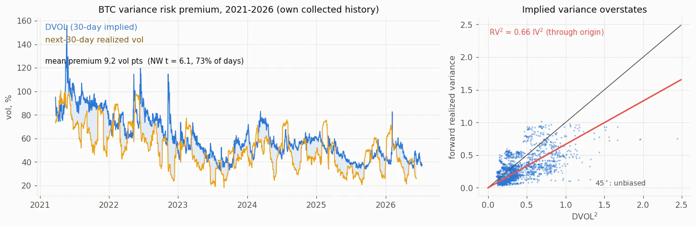
  • 9.2 vol pts measured result BTC variance risk premium, t = 6.1 DVOL vs next-30-day realized vol, 2021–2026; Newey–West t = 6.1, positive on 73% of days
  • 157 + 62 passing check C++ and Python tests Green under release and ASan/UBSan (TSan on the threaded subset), plus 62 Python tests; ~20k lines of C++ and Python
  • 23.9M paths/s measured result Monte Carlo, 8 threads 12-fixing Asian, 65k paths, 8 threads on an M-series machine (4 performance cores; the 8-thread point uses efficiency cores); 5.6M paths/s on 1 thread

Problem

Pricing code is only useful if its numbers can be trusted: bump-and-reprice greeks are slow and noisy, the plain Black formula loses relative precision in the far wings, and surfaces fitted to noisy market quotes can admit arbitrage. Each of those failure modes needs a check stronger than the code under test.

Approach

Header-only C++23 core: Black–Scholes analytics; a tape-based AAD engine (structure-of-arrays arena, expression templates, per-thread tapes, implicit-function-theorem nodes, Cholesky adjoint, forward-over-reverse second order); theta-scheme and Heston ADI PDE solvers; a Savine-style model/product Monte Carlo engine with path-wise AAD, Sobol–Owen QMC, Giles MLMC and Longstaff–Schwartz with Andersen–Broadie bounds; vol-surface code (LBR-architecture implied vol, exact-KKT SVI, arbitrage-free SSVI, Dupire local vol, Heston COS calibration); and a rough Bergomi simulator. pybind11 exposes the core to a Python layer, where a pipeline turns one Deribit snapshot into a certified arbitrage-free surface (an example systemd timer covers daily runs) and research code runs the roughness, variance-risk-premium and hedging studies. A separate, self-contained collector daemon snapshots Deribit BTC/ETH options, futures, index and DVOL to zstd Parquet every 5 minutes on a VPS. Correctness is checked against stronger references: 50-digit mpmath goldens, QuantLib as an external referee, exact-but-slow internal oracles (Broadie–Kaya exact simulation, exact-fBM Cholesky, brute-force polytope search), and no-arbitrage property tests on the Black–Scholes, PDE, Heston and rough-Bergomi pricers. Tolerances are derived from stated error models, stochastic tests are seeded, and CI runs GCC 14 and Clang 18 in Debug+ASan/UBSan and Release, plus a Clang 18 TSan job.

Result

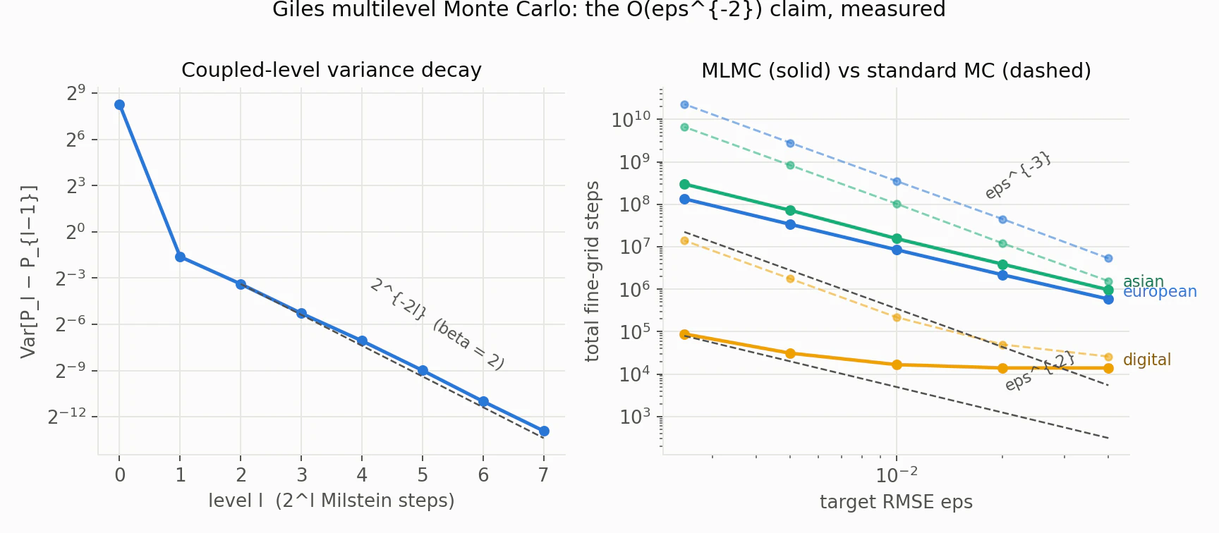
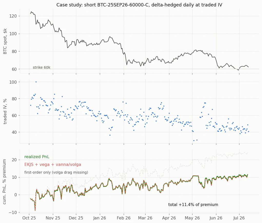
All seven phases are complete, each with a written report in docs/. Measured: a 500-input AAD gradient at 2.83× the cost of one pricing; implied-vol inversion that round-trips 50-digit golden prices to 2e-13 relative error, wings included; MLMC cost scaling as ε−1.96 on a European call (170× cheaper than standard Monte Carlo at ε = 0.0025); and a Dupire round trip on the fitted market surface within ±3.9 bp of vol inside 2.5 sd of ATM. On Deribit BTC data it estimates roughness Ĥ ≈ 0.13 from 3 years of daily realized variance and a mean variance risk premium of 9.2 vol pts (2021–2026, Newey–West t = 6.1), and explains a short real option’s 9-month delta-hedged PnL to within 0.3% of premium once vanna/volga terms are added.

Highlights

  • AAD: a 500-input gradient (250 Black–Scholes options) costs 2.83× one pricing (36.1 µs vs 12.8 µs), 377× faster than central bumps; per-thread tapes TSan-clean
  • Monte Carlo: 23.9M paths/s on 8 threads (12-fixing Asian, M-series); Giles MLMC cost ∝ ε−1.96 vs ≈ε−3, 170× cheaper at ε = 0.0025 (European call)
  • Implied vol (LBR architecture): worst 2e-13 relative price round trip on 50-digit golden prices, wings included; at most 10 evaluations on the test grid
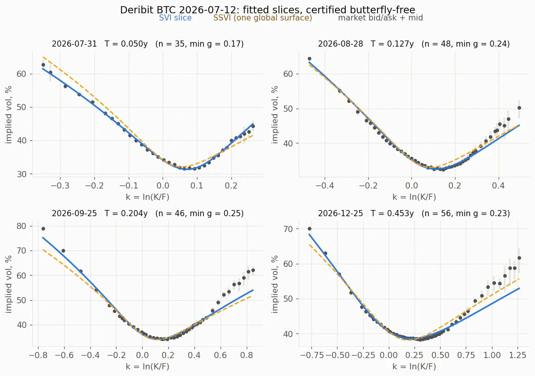
  • Deribit BTC snapshot → exact-KKT SVI slices → certified arbitrage-free SSVI; a Dupire round trip on it stays within ±3.9 bp of vol inside 2.5 sd of ATM
  • BTC data: noise-corrected roughness Ĥ ≈ 0.13 (3 y of daily realized variance); mean variance risk premium 9.2 vol pts over 2021–2026, Newey–West t = 6.1
  • 157 C++ tests (release, ASan/UBSan; TSan on the threaded subset) and 62 Python tests; analytics checked against 50-digit mpmath goldens and QuantLib (< 1e-10)

Lab note

First-order attribution of a short BTC call, delta-hedged daily for 9 months, missed by 13% of premium; adding vanna/volga rows closed it to 0.3%.

Deribit collector
Self-contained Python daemon (systemd unit; deployed on a VPS): BTC/ETH option chains, futures, index and DVOL every 5 min → zstd Parquet (~2 GB/month)
to Committed market data — live snapshot; history fetched via the same API client
to Surface pipeline — one snapshot per run (daily timer: example config)
Committed market data
870-row live options snapshot, 5.3 y hourly DVOL, 3 y daily realized variance, 5.7 y daily spot; tests and figures never need the network
to Python research layer — DVOL, RV, spot, option candles
Surface pipeline
run_daily: parity-regressed forward + discount per expiry → LBR implied vols (OTM, two-sided) → exact-KKT SVI slices → arb-free SSVI; arbitrage scanner; dated JSON + Parquet
to Python research layer — fitted slices → skew study
to pybind11 seam — LBR IVs, SVI/SSVI fits
Python research layer
Roughness estimators, numpy-MLP rBergomi surrogate, variance-risk-premium and hedging studies
to pybind11 seam — rBergomi MC, hedge backtests
pybind11 seam
import deriv — C++ entry points, NumPy-vectorized where it matters
to C++23 pricing core — calls
C++23 pricing core
Header-only: Black–Scholes, LBR/SVI/SSVI/Dupire, Heston CF/COS/ADI, PDE, Monte Carlo (QMC, MLMC, LSMC), rough Bergomi, hedge ledger
AAD engine
Arena tape + expression templates, per-thread tapes, checkpointing, IFT nodes, Cholesky adjoint, forward-over-reverse second order
to C++23 pricing core — MC greeks, calibration Jacobians, IFT greeks
Oracles & test gates
50-digit mpmath goldens, QuantLib referee, exact-but-slow internal oracles, no-arbitrage property tests; 157 C++ + 62 Python tests
to C++23 pricing core — reference tests on each pricer
Fig. 3a — Architecture. Main path: Deribit collector → Surface pipeline → pybind11 seam → C++23 pricing core.
Four of twelve Deribit BTC implied-volatility smiles from the 2026-07-12 snapshot plotted against log-moneyness, with market bid/ask bars and mids, fitted SVI slices (solid) and a single global SSVI surface (dashed)
Deribit BTC options snapshot (2026-07-12): exact-KKT SVI slices and one certified arbitrage-free SSVI surface against market bid/ask; 4 of 12 expiries shown.
BTC DVOL implied vol vs next-30-day realized vol from 2021 to 2026, and a scatter of forward realized variance vs DVOL squared with a fitted line below the 45-degree line
BTC variance risk premium, 2021–2026: mean 9.2 vol pts, Newey–West t = 6.1, positive on 73% of days.
Left: multilevel Monte Carlo level variance decaying along a 2^-2l guide; right: total cost vs target RMSE for MLMC (solid) and standard Monte Carlo (dashed) for European, Asian and smoothed-digital payoffs
Giles MLMC vs standard Monte Carlo on three payoffs. European call: cost ∝ ε−1.96 vs ≈ε−3, 170× cheaper at ε = 0.0025.
Short BTC-25SEP26-60000-C delta-hedged daily: BTC spot, traded implied vol, and cumulative PnL with realized, full attribution and first-order-only lines
A short position in a real Deribit BTC call, delta-hedged daily for 9 months: attribution closes to 0.3% of premium once vanna/volga rows are added (13% with first-order terms only).
Fig. 3b — Four of the figures committed to the repo’s docs/figures, reproduced as published.

Limits

Eigen, Catch2 and pybind11 dependencies; no Dupire stage in the pipeline.

Stack

  • C++23
  • CMake presets
  • Eigen 3.4
  • Catch2
  • Google Benchmark
  • pybind11
  • Python
  • NumPy
  • PyArrow / Parquet (zstd)
  • httpx
  • mpmath (50-digit goldens)
  • QuantLib (test referee)
  • systemd
  • GitHub Actions (GCC 14, Clang 18)
  • ASan / UBSan / TSan

Numbers traced to derivatives-engine @ 50d831c.

Sources

  1. 2.83× 500-input portfolio gradient | 2.83× primal (36.1 µs vs 12.8 µs; target was 3–5×) derivatives-engine / docs/phase1.md @ 50d831c
  2. 9.2 vol pts The BTC variance risk premium, 2021–2026: 9.2 vol pts, Newey–West t = 6.1 derivatives-engine / README.md @ 50d831c
  3. 157 + 62 157 C++ tests green under release and ASan/UBSan (TSan on the threaded subset), 62 Python tests, ~20k lines. derivatives-engine / README.md @ 50d831c
  4. 23.9M paths/s engine throughput (12-fixing Asian, M-series) | 5.6M paths/s (1 thread) → 23.9M (8 threads) derivatives-engine / docs/phase3.md @ 50d831c
  5. Lab note short BTC-25SEP26-60000-C over 284 days: +11.4% of premium; full attribution gap 0.3% of premium (first-order only: 13%) derivatives-engine / docs/phase6.md @ 50d831c

LineWatch

Crowdsourced NYC wait times with 12-hour LightGBM line forecasts and P10–P90 bands

SYNTHETIC DATA STATUS — v0.1.0 — runs locally via Docker Compose on synthetic data; not publicly deployed

SIM · the app’s synthetic daily curves, 1 h per second

  • 12 h design value P10–P90 forecasts Default for the API and the UI chart (the API accepts 1–24 h); LightGBM point forecast with a P10–P90 band from α = 0.10 / 0.90 quantile models
  • 53 design value real NYC venues, synthetic reports Approximate coordinates; paired with ~45 days of synthetic wait reports from per-category daily curves. Optional Google Places ingest covers 15 neighborhood pivots
  • 3.5 σ design value MAD outlier gate at ingest MAD-based; needs ≥ 4 recent reports and never flags deviations < 15 min. Flagged reports are stored but excluded from live medians, trend signals and training

Problem

Lines at NYC bars, clubs and restaurants change hour to hour, and crowdsourced wait reports are noisy and easy to game. A useful app needs a live number that a single wild report barely moves. It also needs a forecast judged the way it will be used, rolling forward in time, not by row-wise cross-validation.

Approach

FastAPI finds nearby venues and their live waits in one PostGIS query: a GiST-indexed ST_DWithin search whose CTEs take medians over non-outlier reports, counting each signed-in reporter once. A second batched query and a single LightGBM call then predict a current wait for every venue, and the response is cached in Redis and purged whenever a report lands. Each new report is screened by a MAD-based outlier gate (3.5 robust SDs; at least 4 recent reports needed; deviations under 15 min never flagged), stored with its flag, then appended to a capped Redis Stream and pushed to browsers over SSE with Last-Event-ID replay. A LightGBM regression model builds the 12-hour curve from NYC-local time features, venue attributes and rolling trend features that exclude each row’s own label, trained on non-outlier reports with a chronological last-15% holdout and optional Optuna TPE tuning; α = 0.10 / 0.90 quantile models give the P10–P90 band, and a manifest with feature names and a FEATURE_VERSION makes the predictor refuse a mismatched model and fall back to a heuristic instead of mispredicting. A walk-forward backtest retrains per fold, scores the model against persistence, heuristic and climatology baselines and checks P10–P90 calibration; once it has been run, its report is served at /stats/model and shown in the UI.

Result

docker compose up --build runs migrations, seeds 53 NYC venues, generates ~45 days of synthetic reports and trains the model (skipped on later boots if the saved model still matches the feature schema). On pushes to main and on pull requests, CI runs migrate → seed → generate → train, a miniature walk-forward backtest (2 folds over 3 days of synthetic data) and the full pytest suite against PostGIS and Redis service containers, plus frontend lint, typecheck and build. No backtest results are committed and all training data is synthetic, so no accuracy figures are claimed.

Highlights

  • 12-hour forecast per venue: a LightGBM regression curve plus α = 0.10 / 0.90 quantile models for the P10–P90 band, cached 60 s in Redis.
  • Walk-forward backtest: retrain on reports before each origin T, predict (T, T+12 h] using only what a live server knew at T; 3 baselines + P10–P90 coverage.
  • Robust live waits: medians, not means; reports > 3.5 MAD-based SDs from the venue’s recent consensus are stored but excluded from medians, trends and training.
  • Nearby venues + live medians in one PostGIS query (GiST-indexed ST_DWithin, median CTEs, no N+1); a report purges 30 s nearby + its venue’s 60 s forecast keys.
  • Live map over SSE from a capped (~1,024-entry) Redis Stream; reconnects replay missed events via Last-Event-ID, while 30 s polling stays the source of truth.
  • One canonical feature order for training and serving, NYC-local time features and a chronological last-15% holdout; mismatched models are refused at load.

Lab note

Mean band width is reported beside P10–P90 coverage, because coverage alone is gameable with arbitrarily wide bands.

Next.js + Mapbox GL
Markers colored by wait band, pulse on live events; Recharts forecast with P10–P90 band; SWR polling + EventSource
to FastAPI — REST polling + POST /reports
FastAPI
/venues, /reports (10/min/IP), /predictions, /stats, /events/stream; X-Cache, X-Query-Ms (cache misses) and X-Request-Ms headers
to Outlier gate — new report
to PostGIS — ST_DWithin + median CTE
to Redis — cache · purge · XADD
to Next.js + Mapbox GL — SSE /events/stream
to LightGBM predictor — batched feature rows
Outlier gate
MAD-based robust z > 3.5 vs the last 90 min of non-outlier reports; needs ≥ 4 priors; deviations < 15 min never flagged
to PostGIS — insert with is_outlier
PostGIS
venues (GiST geography index) + wait_reports; ST_DWithin + live-median CTE in one query
to Train + backtest — non-outlier reports
Redis
Endpoint-shaped cache keys (30–60 s TTL); nearby and forecast keys purged per report; capped events:reports Stream (~1024)
to FastAPI — XREAD from Last-Event-ID
LightGBM predictor
Regression + P10/P90 quantile boosters, batched predict per curve; manifest feature_names + FEATURE_VERSION guard; heuristic fallback
Train + backtest
Leakage-free trend features, chronological last-15% holdout, optional Optuna TPE; walk-forward backtest vs 3 baselines
to LightGBM predictor — boosters + manifest
to FastAPI — backtest report → /stats/model
Seed data
53 real NYC venues + ~45 days of synthetic reports; optional Google Places ingest (15 pivots)
to PostGIS — venues + reports
Fig. 4a — Architecture. Main path: Next.js + Mapbox GL → FastAPI → Outlier gate → PostGIS.
Walk-forward backtest, per fold
StepWhat happens
TrainRetrain on every report strictly before the fold origin T
PredictEvery report in (T, T+12 h], using only what a live server had at T
ScoreAgainst persistence, heuristic-fallback and climatology baselines; P10–P90 coverage vs the nominal 80%, with mean band width
In CIA miniature run: 2 folds over 3 days of synthetic data
Fig. 4b — Walk-forward protocol: retrain before each origin T, predict (T, T+12 h] using only what was known at T. Protocol only: no results are committed.

Limits

Synthetic and undeployed.

Stack

  • Python 3.12
  • FastAPI
  • Pydantic
  • SQLAlchemy 2
  • GeoAlchemy2
  • Alembic
  • PostgreSQL 16 + PostGIS 3.4
  • Redis 7 (cache + Streams)
  • Server-Sent Events
  • LightGBM
  • Optuna
  • scikit-learn
  • pandas
  • NumPy
  • slowapi
  • structlog
  • Next.js 15 (App Router)
  • React 19
  • TypeScript
  • Tailwind CSS
  • Mapbox GL JS
  • Recharts
  • SWR
  • Docker Compose
  • GitHub Actions
  • pytest
  • ruff
  • Google Places API (New)

Numbers traced to line-watch @ ab9602e.

Sources

  1. 12 h horizon_hours: int = Query(default=12, ge=1, le=24), line-watch / backend/app/api/predictions.py @ ab9602e
  2. 53 Seed 53 real NYC venues (app/scripts/seed_venues.py). line-watch / README.md @ ab9602e
  3. 3.5 σ OUTLIER_ROBUST_Z = 3.5 line-watch / backend/app/services/reports.py @ ab9602e
  4. Lab note mean band width (sharpness), because coverage alone is gameable with arbitrarily wide bands line-watch / README.md @ ab9602e

ShotSense

Photo-curation prototype: 0–100 style-match scores on a ViT-B/32 implemented layer by layer in PyTorch

PROTOTYPE STATUS — Prototype: training loop and API implemented; no trained checkpoint or evaluation results published

SIM · illustrative data, not model output

  • 128-d design value style space, 0–100 match 512→384→256→128 MLP head, L2-normalized; training loss combines triplet, orthogonality and attribute terms
  • ~87M design value frozen ViT-B/32 parameters Implemented layer by layer in PyTorch and loaded with CLIP weights; only the small heads train
  • 5–10 design value reference photos per look The README’s suggested count (the API accepts 2 or more); combined into one prototype that each candidate is scored against, 0–100

Problem

Directing a photography team means communicating a target look before a shoot, then culling hundreds of photos manually to find the ones that match it. ShotSense starts from the premise that off-the-shelf CLIP embeddings mix what is in a photo with how it looks, so two shots with the same moody aesthetic but different subjects (portrait vs. landscape) can sit far apart.

Approach

Implements ViT-B/32 module by module in PyTorch: a Conv2d patch embedding into 49 tokens plus [CLS] at 768-d, then 12 pre-norm blocks with 12-head attention, which uses PyTorch’s scaled_dot_product_attention by default and an explicit softmax(QKᵀ/√d) path when attention maps are requested. OpenAI CLIP weights load through a key-remapping loader, and the ~87M-parameter backbone stays frozen. A 512→384→256→128 MLP maps the backbone’s 512-d embedding onto an L2-normalized 128-d style space, and the training objective weights three terms 1.0 / 0.5 / 0.3: cosine-distance triplets with margin 0.3, a Frobenius-norm penalty on the cross-correlation between style vectors and the backbone embeddings (used as the content signal), and MSE on six attribute heads against pseudo-labels computed from pixel statistics. Augmentation is deliberately geometric-only (random crop, horizontal flip). At inference, an attention module (key/value projections plus a query vector) combines the reference style vectors into one unit-norm prototype, and each candidate is scored by cosine similarity to it, rescaled to 0–100. A FastAPI service exposes project setup, reference upload, batch ranking, per-attribute gap analysis and a rule-based style guide.

Result

A runnable prototype: a training loop (AdamW, cosine LR schedule, gradient clipping at 1.0, checkpointing, a validation triplet retrieval-accuracy metric) and a FastAPI service for project setup, reference upload, batch ranking, per-photo gap analysis and style-guide generation. Only the small heads train; the ~87M-parameter ViT backbone stays frozen. The repo publishes no trained checkpoint or evaluation numbers, so no accuracy figure is claimed.

Highlights

  • ViT-B/32 implemented layer by layer in PyTorch: 49 patch tokens + [CLS] at 768-d through 12 pre-norm blocks × 12 heads; OpenAI CLIP weights loaded by key remapping
  • 128-d unit-norm style space from a 512→384→256→128 MLP head; 3-term training loss (triplet with margin 0.3, orthogonality, attributes) weighted 1.0/0.5/0.3
  • Orthogonality term: Frobenius norm of the style × backbone-embedding cross-correlation, aimed at keeping style vectors uncorrelated with content
  • 6 attribute heads (warmth, contrast, saturation, brightness, sharpness, grain) supervised by pseudo-labels from pixel statistics instead of manual labels
  • FastAPI flow: 5–10 suggested references → style prototype → candidates ranked 0–100 → per-attribute gap labels (±0.1) and a rule-based style guide

Lab note

No color jitter in augmentation: it would destroy the style signal the model is learning.

Photos 224×224
CLIP-normalized; training uses geometric-only augmentation (random crop, horizontal flip)
to ViT-B/32 backbone — image tensor
ViT-B/32 backbone
Conv2d patch embed → 49 tokens + [CLS] at 768-d → 12 pre-norm blocks × 12 heads → [CLS] projected to 512-d; OpenAI CLIP weights via key remapping; ~87M params, frozen
to Style head → 128-d — 512-d embedding
to 3-part loss (training) — content signal (orthogonality)
Style head → 128-d
MLP 512→384→256→128 with LayerNorm + GELU; output L2-normalized onto the unit sphere
to 6 attribute heads — 128-d style vector
to 3-part loss (training) — anchor / positive / negative
to Few-shot prototype — reference vectors
to Score 0–100 — candidate vectors
6 attribute heads
warmth, contrast, saturation, brightness, sharpness, grain; sigmoid outputs in [0, 1]
to 3-part loss (training) — vs pseudo-labels
to FastAPI service — attribute gaps, style guide
3-part loss (training)
1.0 × cosine triplet (margin 0.3) + 0.5 × orthogonality (Frobenius norm of style × backbone-embedding cross-correlation) + 0.3 × attribute MSE vs pixel-statistic pseudo-labels
Few-shot prototype
Attention weights from key similarity among the references plus a query vector; weighted sum of value projections, L2-normalized into one prototype
to Score 0–100 — prototype
Score 0–100
Cosine similarity to the prototype, rescaled (cos + 1) / 2 × 100; candidates sorted
to FastAPI service — ranked scores
FastAPI service
projects · references · upload & rank · analyze (per-attribute gaps, ±0.1) · style guide
Fig. 5a — Architecture. Main path: Photos 224×224 → ViT-B/32 backbone → Style head → 128-d → Few-shot prototype → Score 0–100 → FastAPI service.
Parameters
PartParametersTraining
ViT-B/32 backbone87,848,448frozen
Style, attribute and prototype heads371,526trainable
Loss: L = 1.0·L_triplet + 0.5·L_orth + 0.3·L_attr
TermWeightWhat it measures
L_triplet1.0cosine-distance triplets, margin 0.3
L_orth0.5Frobenius norm of the style × backbone-embedding cross-correlation
L_attr0.3attribute MSE against pixel-statistic pseudo-labels
Fig. 5b — Drawn to scale: only the heads train.

Limits

No checkpoint.

Stack

  • PyTorch
  • torchvision
  • OpenCLIP (weight loading)
  • FastAPI
  • Uvicorn
  • Pydantic
  • NumPy
  • Pillow

Numbers traced to shotsense @ ee5ecb5.

Sources

  1. 128-d 128-dim Style Vector (L2-normalized) shotsense / models/style_encoder.py @ ee5ecb5
  2. ~87M ViT Backbone | ~87M | ✗ (frozen) shotsense / README.md @ ee5ecb5
  3. 5–10 Define your style — Upload 5-10 reference photos that capture the vibe you want shotsense / README.md @ ee5ecb5
  4. Lab note # NOTE: We intentionally do NOT use ColorJitter or style-altering # augmentations, because those would destroy the style signal shotsense / data/dataset.py @ ee5ecb5

market-maker

Avellaneda–Stoikov market maker simulated on recorded and live Binance L2 order books

NEGATIVE RESULT STATUS — v0.2.0 (Aug 2026); hour-tape results reproducible from committed tapes

SIM · skew exaggerated for legibility

  • 95% CI < 0 measured result AS loss on BTCUSDT Moving-block bootstrap, 1,000 resamples, seed 7; walk-forward calibration, 50 ms latency, 1 bp maker fee. AS − naive: not significant on either hour tape.
  • 0.0013 bp measured result BTCUSDT spread vs a 1 bp fee Caps touch capture at ~0.0007 bp against a 1 bp maker fee; the AS loss is significant (95% CI excludes zero)
  • 295 fills passing check identical, live vs replay BTCUSDT live session vs recorded-order replay of its own tape: identical fills and metrics (property pinned by tests; re-verified on both hour tapes)
  • 72,192 measured result L2 events in one live-recorded hour L2 depth + trades incl. 36,225 prints; one unbroken 60-minute session recorded 2026-08-29, replayed event by event

Problem

A market-making backtest’s results depend heavily on its fill model. Filling quotes at the touch with no queue or latency, with parameters fitted on the same data being traded, can book maker profits that would not exist live. The question is whether the canonical Avellaneda–Stoikov quoter earns the spread on real crypto order books once those effects are modeled, answered with confidence intervals rather than a single PnL number.

Approach

Records Binance spot depth (a REST snapshot seed plus 100 ms diff-depth and aggTrade streams) with update-ID continuity checks and automatic resync, then replays the JSONL tape event by event. In the reported runs, σ (a realized-variance estimator on the irregular event grid) and the fill intensity λ(δ)=A·e−kδ refit walk-forward every 30 s from a trailing 300 s window; λ is fitted by count-weighted log-OLS on trade-through opportunities at several distances from mid, with sweep-print coalescing and a scale-aware fallback (k = 1/median print distance) when the fit degenerates. The Avellaneda–Stoikov quoter centers on reservation = mid − q·γσ²(T−t) + (microprice − mid) with half-spread ½γσ²(T−t) + (1/γ)·ln(1+γ/k), with T−t held at a rolling 60 s horizon in the reported runs; quotes are tick-snapped, passive and inventory-capped, and run head-to-head against a naive constant-spread baseline on the same tape. A price-time-priority engine models visible queue-ahead (size drops not explained by trades count as cancellations ahead of the quote, the optimistic convention), print-size-bounded trade-through fills, order latency with post-only rejection at arrival, and cancel-in-flight pick-off, and books maker fees, markouts and adverse selection per fill. Results carry moving-block bootstrap 95% CIs and a paired AS-minus-naive test. The same TradingSession drives live shadow trading on the real-time book, with simulated fills and no orders sent.

Result

The evaluation uses two unbroken 60-minute tapes live-recorded on 2026-08-29 (BTCUSDT and TRXUSDT), walk-forward calibration, a 1 bp maker fee, 50 ms order latency and deliberately tiny sizing. On BTCUSDT the result is negative: the one-tick 0.0013 bp spread caps touch capture at ~0.0007 bp against a 1 bp fee, and the AS loss is significant at 95% (the bootstrap CI excludes zero). The paired AS-minus-naive difference is not significant at 95% on either tape, and both hour-tape results regenerate from the committed tapes with the README’s commands.

Highlights

  • 72,192 live-recorded BTCUSDT L2 events (36,225 prints, one unbroken 60-minute session) replayed event by event; σ/A/k refit walk-forward every 30 s.
  • Price-time-priority fill engine: visible queue-ahead, print-size-bounded trade-throughs, 50 ms order latency (reported runs), post-only rejection at arrival.
  • Live shadow trading on the real-time Binance book through the backtester’s TradingSession: simulated fills, no orders sent; tape replays give identical fills.
  • BTCUSDT negative result: a one-tick 0.0013 bp spread caps touch capture at ~0.0007 bp vs a 1 bp fee; the AS loss is significant at 95%.
  • Moving-block bootstrap (1000 resamples, 95% CIs) plus a paired AS-minus-naive test on the same tape; the difference is not significant on either hour tape.

Lab note

One 10-lot print could fill 13 lots across price levels; fixed by sharing one fill budget between trade-through and at-price fills.

Binance market data
Public REST depth snapshot + diff-depth @100ms + aggTrade WebSocket streams
to Stream sync + recorder — REST snapshot + WS streams
Stream sync + recorder
data_sources.py: documented sync recipe, update-ID continuity checks, resync from a fresh snapshot, bounded reconnects; flushes every event as it arrives
to JSONL L2 tape — record-binance-depth / --tape-output
to TradingSession — paper-trade (live shadow)
JSONL L2 tape
data.py: snapshot / l2update / trade events; replayed timestamp-sorted or in recorded wire order (--replay-order)
to TradingSession — backtest replay
TradingSession
backtest.py + orderbook.py: one event-by-event loop shared by backtest and live paper-trade; marks PnL to mid
to Walk-forward calibration — every event (walk-forward observer)
to AS quoter vs naive baseline — book + inventory
to Metrics + bootstrap — fills + PnL path
Walk-forward calibration
calibration.py: realized-variance σ; λ(δ)=A·e−kδ via count-weighted log-OLS; scale-aware fallbacks
to AS quoter vs naive baseline — σ, A, k refits
AS quoter vs naive baseline
strategy.py: reservation mid − q·γσ²(T−t) + microprice signal; half-spread ½γσ²(T−t) + (1/γ)ln(1+γ/k)
to Price-time-priority engine — post-only bid/ask quotes
Price-time-priority engine
matching.py: visible queue-ahead, print-bounded trade-through fills, latency, post-only rejection, pick-off window
to TradingSession — fills
Metrics + bootstrap
metrics.py + stats.py: markouts, adverse selection, Sharpe, drawdown; block-bootstrap 95% CIs, paired AS−naive test
Fig. 6a — Architecture. Main path: Binance market data → Stream sync + recorder → JSONL L2 tape → TradingSession → AS quoter vs naive baseline → Price-time-priority engine.
BTCUSDT hour tape. Sizing is deliberately tiny: the signs and intervals are the result, not the dollar magnitudes.
QuantityValue
Maker fee1 bp
Maximum touch capture (one-tick spread)~0.0007 bp
AS final PnL, 95% CI−$1.788 [−2.360, −1.219]
AS − naive, 95% CI+$0.028 [−0.050, +0.106]
Fig. 6b — Drawn to scale. AS loss: 95% CI excludes zero. AS − naive: not significant on either hour tape.

Limits

Simulated fills. TRXUSDT per-fill economics omitted: its runs used a tick 10× finer than the exchange’s.

Stack

  • Python 3.10+
  • Standard library only (core)
  • asyncio
  • websockets (optional, live data)
  • matplotlib (optional, figures)
  • Binance Spot REST + WebSocket market data
  • unittest
  • ruff

Numbers traced to market-maker @ 9c201af.

Sources

  1. 95% CI < 0 The AS loss itself is significant (the CI excludes zero) market-maker / README.md @ 9c201af
  2. 0.0013 bp BTCUSDT’s time-weighted spread on this tape is one tick = 0.0013 bp of price, so the maximum touch capture is ~0.0007 bp against a 1 bp fee. market-maker / README.md @ 9c201af
  3. 295 fills The live paper sessions and recorded-order replays of their own tapes produce identical fills and metrics market-maker / README.md @ 9c201af
  4. 72,192 BTCUSDT L2 depth + trades, 72,192 events (36,225 prints) over 60 minutes market-maker / README.md @ 9c201af
  5. Lab note one print could fill more than its own volume across price levels (10-lot print → 13 lots filled) market-maker / reports/RESULTS.md @ 9c201af

Graphics paused · reconnecting…